 Svenesis.org
17 August 2026 · 🔭 Astronomy
Why have I been shooting 300 seconds all this time? – the optimal sub length, measured and calculated
Three hundred seconds per frame. The number came with the profile I inherited; it turns up in almost every article I have written – filters, dithering, calibration – and I have never justified it. Which sits badly with my own principle that an inherited number is not yet a checked number.
This morning I finally got round to it. A holiday house in Denmark, my son still asleep, my wife out walking, me at the dining table with the laptop – and in Texas it is the middle of the night. For once seven time zones are an advantage: what is mid-morning before breakfast here is the best hour of the night there. With the full version of SharpCap I spent two sessions taking the measurements this calculation had been missing.
The result first: a single number for every filter is wrong. For luminance 300 seconds is generous; 60 would do. For R, G and B it fits, though 180 would be the better compromise. In narrowband it is too short – at 600 seconds I get as much out of the same night as a night a quarter longer would otherwise give me.
And because the sky rate is now measured, the calculation can be turned around: for Starfront it yields a sky of about SQM 21.9, which is Bortle 2 – derived further down.
What this is about
Total time is not the question: five hours are five hours, whether in 60 frames of 5 minutes or 10 of 30. The one thing that differs is read noise – it arises afresh with every readout, regardless of how long the exposure was. Sixty subs, 60 helpings of it; ten subs only ten.
So longer is always better. The only question is when it stops paying off – namely as soon as the photon noise of the sky swamps the read noise. If a pixel counts N photons on average, that number varies by √N; once that variation exceeds the one from the electronics, a little more electronic noise no longer matters.
Robin Glover, the author of SharpCap, cast this into an equation:
t = C · R² / P
t is the optimal sub length, R the read noise in electrons, P the rate at which the sky delivers electrons per pixel per second.
C depends only on how much added noise you accept: C = 1/((1+E)²−1). At five per cent that is 1/(1.05²−1) = 9.75, at ten per cent 4.76.
Two things are packed into it. Read noise enters as a square – half the noise, a quarter of the time. And the sky enters linearly – a dark sky calls for longer subs, and a narrowband filter turns that into the extreme case.
So there are two numbers to obtain.
R – the read noise of my camera
This one I did not have to estimate. SharpCap has a sensor analysis built in that measures the whole response curve from around 900 frames against an evenly lit surface. My flat panel is ideal for it: cover shut with the light on for the bright frames, cover shut with the light off for the darks, and the brightness adjustable in 4096 steps.
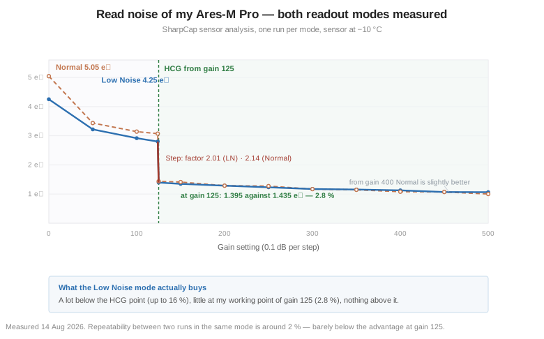
2.80 electrons down to 1.395 – a factor of 2.01, in a single step. The high-conversion-gain switchover point of the IMX533. I run gain 125 anyway, for other reasons – what I never worked out there is that this one setting cuts the required sub length to a quarter, because R enters as a square.
In passing, that also makes gain 124 the worst setting on the whole curve: the highest noise immediately before the step and the lowest dynamic range. One step off costs you twice.
From here on I use R = 1.395 e⁻, the figure in the Low Noise readout mode. Whether that mode buys anything at all is in the appendix, along with the full curve.
P – my sky
For a long time this was the weak spot in the calculation. In the flat panel article I estimated 0.8 electrons per pixel per second in the luminance filter, derived from SQM 21.9, 81 mm of aperture and 2.03 ″/px – and divided by seventy for narrowband, because the 4.5 nm filters pass roughly that much less.
Although I have to say where those 21.9 came from: nowhere. Starfront classify the site as Bortle 1 and publish no SQM figure; my own rig page quotes the range SQM 21–22. The 21.9 was a pick from inside that range, measured by nobody. So the estimate rested on an estimate – which is exactly why it is worth turning around.
Now it is measured. SharpCap's Smart Histogram gives the rate directly, one run per filter:
| Filter | Sky rate |
|---|---|
| L | 0.68 e⁻/px/s |
| B | 0.19 |
| G | 0.16 |
| R | 0.14 |
| Hα · OIII · SII | 0.01 |
Two things stand out.
My estimate held up. 0.68 instead of 0.8 in the luminance filter – fifteen per cent off, for a number derived from an SQM reading and an aperture.
And the factor of 70 cannot be shown. 0.68 divided by 0.01 is 68, yes – but the 0.01 is what SharpCap prints to two decimal places. Anything between 0.005 and 0.015 can sit behind it, which puts the ratio somewhere between 45 and 136. The assumed 70 fits comfortably inside that – and that is all the measurement says. The arithmetic roughly agrees: some 300 nm of luminance band against 4.5 nm of narrowband is 67, though the sky does not radiate evenly across the band.
Two decimal places is where narrowband ends: all three filters read 0.01, so Hα, OIII and SII cannot be told apart. What that vagueness means for the recommendation comes further down. What matters in a measurement like this, and how to manage it without a SharpCap licence, is in the appendix.
What the measurement says about my sky
So far the calculation only ran one way: sky brightness in, electrons per second out. Now the rate is measured – so it can be turned around. What comes out is the number you otherwise only get from light-pollution maps or from the operator’s website, this time from my own equipment:
21.9
SQM in mag/arcsec²
Bortle 2
sky class
How it is calculated
A star of magnitude V = 0 delivers about 1,000 photons per second, square centimetre and ångström above the atmosphere. Across the 880 Å width of the V band that is 8.8 · 105 photons per second and square centimetre. And “SQM 21.9” means nothing more than this: every square arcsecond of sky glows as brightly as a star of magnitude 21.9. The rest is geometry and throughput:
P = 8.8 · 105 · 10−0.4 · SQM · A · Ω · η · k
| Quantity | Value | where it comes from |
|---|---|---|
| A – collecting area | 51.5 cm² | 81 mm clear aperture, refractor, no obstruction |
| Ω – solid angle per pixel | 4.12 arcsec² | (2.03 ″/px)² |
| η – throughput | 0.61 | quantum efficiency of the IMX533 averaged over the L band (~0.70), times optics and filter (~0.87) |
| k – bandwidth | 3.4 | the luminance filter is a UV/IR block, roughly 390 to 690 nm – against the 880 Å of the V band |
| P – sky rate | 0.68 e⁻/px/s | measured, see above |
Solved for SQM, with the measured 0.68 substituted in: 21.89 magnitudes per square arcsecond.
How solid the number is
A and Ω are hard, P is measured. The soft parts are η and k – both assumptions, not measurements. So here is the range rather than a decimal place that does not exist:
| Assumption | η | k | SQM |
|---|---|---|---|
| pessimistic | 0.55 | 3.0 | 21.64 |
| assumed | 0.61 | 3.4 | 21.89 |
| optimistic | 0.67 | 3.8 | 22.11 |
So 21.6 to 22.1. Two further things nudge the result upwards. The luminance run sat at 63.5 degrees altitude, not at the zenith – through 1.12 airmasses the background is a shade brighter than at the darkest point of the sky, which makes the estimate conservative. And a real SQM meter measures with its own spectral response over a field many degrees wide, whereas my number comes through a telescope, a filter and a sensor. The two quantities carry the same name, but they do not come from the same instrument.
And what is that in Bortle?
Only the Bortle scale is not a measurement. In Sky & Telescope in 2001, John Bortle described nine classes through visible phenomena and the naked-eye limiting magnitude, not through SQM values – the Sky Quality Meter arrived years later, and Unihedron publishes no mapping of its own to this day. What circulates are later readings, and they differ by up to three tenths of a magnitude. Martin Hochbruck pointed that out to me; the figures in the first version of this article struck him as too strict. Rightly so – so here are all four variants side by side. Pick the one you compare against, and name it:
| Class | Description | Strict variant | Stellarium | Engl. Wikipedia | Martin |
|---|---|---|---|---|---|
| 1 | excellent dark sky | from 21.99 | 21.7 – 22.0 | 21.76 – 22.0 | from 21.85 |
| 2 | typical truly dark sky | 21.89 – 21.99 | 21.5 – 21.7 | 21.6 – 21.75 | – |
| 3 | rural sky | 21.69 – 21.89 | 21.3 – 21.5 | 21.3 – 21.6 | – |
| 4 | rural / suburban transition | 20.49 – 21.69 | 20.4 – 21.3 | 20.8 – 21.3 | to 21.4 |
My measured 21.89 therefore lands in different places: in the strict column it sits exactly on the threshold between class 3 and class 2, in the other three it sits in class 1.
Which variant is the better one cannot be proven, but it can be bounded: the world atlas of light pollution (Falchi et al. 2016) uses 174 µcd/m² for the natural sky, about 22.0 mag/arcsec², and real measurements at pristine sites land between 21.7 and 22.0 because of airglow, moving with the solar cycle. A table demanding at least 21.99 for class 1 therefore calls almost every genuinely dark place on Earth a class 2 – which sits badly with Bortle’s own description, asking for the zodiacal light, the gegenschein and M33 with the naked eye, not for a record reading. I consider the strict column too strict; what holds either way is the measured SQM number, the class is convention.
Starfront advertise “exceptionally dark Bortle 1 skies”. Under three of the four mappings my measurement supports that, under the strictest it would be class 2. The operator quotes no SQM number; the 21–22 on my rig page is the closest thing there is.
Sources of the mappings: Bortle scale (English Wikipedia, after Dark Skies Awareness) · Stellarium manual · AstronomyCalc (strict variant) · Unihedron FAQ · Falchi et al. 2016. Thanks to Martin for the pointer.
Between the two darkest Bortle classes lie one or two tenths of a magnitude, depending on the mapping – little in practice. Between my measured 21.89 and a good rural sky in Germany lies half a magnitude, and that one shows up in every single sub.
A good rural sky in Germany sits somewhere around 21.3 to 21.5. Half a magnitude darker means a good third less sky background per pixel – and, for the same total integration time, roughly a quarter more signal-to-noise. That is exactly why the rig stands in Texas and not here.
As a by-product, the calculation settles an open question from the flat-panel article. There I estimated a rate of 0.8 e⁻/px/s from SQM 21.9; the measured value is 0.68. The difference was not the sky but my throughput assumption at the time: with the values in the table above, SQM 21.9 gives a rate of 0.67 – which is the measured one. So the assumed sky was right – which, for a pick out of the 21–22 range, is partly luck, given that my own derivation is itself only good to a couple of tenths. What was too generous was the assumption about optics and filter width.
The result
Put into t = 9.75 · R² / P:
| Filter | Sky rate | optimal sub length |
|---|---|---|
| Luminance | 0.68 | 28 s |
| B | 0.19 | 100 s |
| G | 0.16 | 119 s |
| R | 0.14 | 136 s |
| Narrowband 4.5 nm | 0.01 | 32 min |
From half a minute to half an hour – a factor of 68, the ratio of the sky rates used. And the colour filters need longer exposures than luminance, because only about a quarter of the light comes through them.
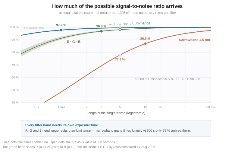
Luminance: 99.5 per cent of what is theoretically possible. Even 60 seconds would sit at 97.7. There is nothing left to gain here.
R, G, B: around 98 per cent. Here too 300 seconds is plenty; 180 would still reach 96 to 97.
Narrowband: 77.9 per cent. That sounds like a small loss, but it is the wrong way to look at it – and the place where I got stuck myself on first reading. So here it is in full.
The yardstick is an infinitely long exposure: there the read noise arises exactly once, and it does not get better than that. With 300-second subs I reach 77.9 per cent of it – at the same total time. And because signal-to-noise grows only with the square root of time, catching up costs not 22 per cent more time but the square of that: 1 ÷ 0.779² = 1.65.
Worked through for one night:
| I collect | 10 hours of Hα in 300-second subs |
| What arrives is the equivalent of | 6.1 hours of perfect exposure |
| For a real 10 hours I would need | 16.5 hours |
So nearly forty per cent of the night is gone – not because anything breaks, but because the read noise of 120 readouts adds up.
| Sub length | % of the maximum | of that thrown away | extra time needed |
|---|---|---|---|
| 300 s | 77.9 % | 39 % | +65 % |
| 600 s | 86.9 % | 25 % | +32 % |
| 900 s | 90.7 % | 18 % | +22 % |
| 1800 s | 95.0 % | 10 % | +11 % |
And what if the 0.01 is off? It could mean anything between 0.005 and 0.015, after all. The recommendation holds regardless:
| actual P | optimum | 300 s | 600 s |
|---|---|---|---|
| 0.005 | 63 min | 66 % | 78 % |
| 0.010 | 32 min | 78 % | 87 % |
| 0.015 | 21 min | 84 % | 91 % |
In all three cases the step from 300 to 600 seconds buys twelve to thirteen percentage points.
Why I am not going to 32 minutes anyway
The formula knows two quantities. Reality knows more, and every one of them argues for shorter frames.
The usual suspect is the mount – the longer the exposure, the more opportunity for a tracking error that no amount of stacking will repair. That can be tested: I took the PHD2 log of the M16 night, 4,412 frames, and cut it into sliding windows of five to sixty minutes. If guiding degrades over time, it has to show up here.
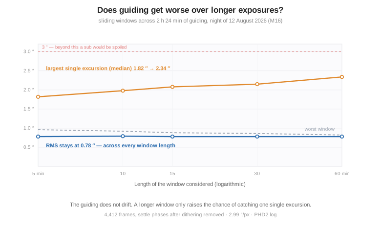
The RMS does not change – 0.78 arcseconds, whether the window covers five minutes or an hour. Only the largest single excursion grows, and across two and a half hours there was not one excursion beyond 3 arcseconds. On that night a 30-minute sub would in fact have been guided more evenly than the worst five-minute window.
So the usual suspect is ruled out. What remains are three other reasons:
The number of frames
This is the hard objection, and it comes out of my own articles: kappa-sigma starts working at about ten frames and becomes reliable beyond twenty. My stacking script only switches to GESDT from 31 frames, and for drizzle it demands 40 dithered subs – which is no luxury given my undersampling of 1.6 pixels per star width. At 32-minute subs I would end up with three per channel per night.
Every lost sub costs more
Satellite, gust, cloud – at five minutes I lose five, at thirty I lose thirty. The problem is not the probability but the stake.
Star saturation
Even at 30 minutes of narrowband the sky fills only a thousandth of the well – the stars do not.
My decision
60 s
Luminance · was 300
180 s
R · G · B · was 300
600 s
Narrowband · was 300
Narrowband: 600 seconds. The loss falls from nearly forty per cent to a quarter, and there are still enough frames left for outlier rejection. Going further buys four percentage points and costs the statistics.
Luminance: shorter, 60 seconds. Still 97.7 per cent, and having fewer burnt-out stars is a gain in itself.
R, G, B: 180 seconds. That puts me at 96 to 97 per cent while giving me two thirds more frames than 300 seconds – and burnt-out stars are especially annoying in the colour channels, because they take the star colours with them. At 60 seconds it would be only 90 to 92 per cent, which is too short.
The theoretical optimum is never the answer. It is the ceiling you weigh your choices against.
Corrections to earlier articles. Working through the numbers, I found four I had given too roughly before:
· The CMOS article and the gain article both give the read noise in HCG mode as “about 1 electron”. Measured, it is 1.395 e⁻. For the formula above that is a factor of two in time.
· In the flat panel article I derived the system gain and saturation from the 73 ke figure: 1.06 e⁻/ADU and 17,300 e⁻. Measured, they are 1.04 e⁻/ADU and 17,040 e⁻.
· The same article carries the estimated sky rate of 0.8 e⁻/px/s in the luminance filter. Measured, it is 0.68.
· In the sampling article I worked with a guiding RMS of 0.62 ″. The night now measured comes in at 0.78 ″, so the FWHM contribution is 1.84 rather than 1.2 arcseconds. It does not change the verdict of “undersampled”, but it does change the error budget.
I worked all of this through, as has become my habit, together with Claude AI.
Appendix A – the second readout mode: does it buy anything?
The Ares series has a second sensor mode, “Low Noise”. Player One explicitly recommends it for deep sky in the manual. It is found here:
| Native driver in N.I.N.A. | Options → Equipment → Camera → Readout mode → Low Noise |
| ASCOM driver | Chooser → Properties → Sensor Mode → Low Noise mode |
Whether it buys anything is disputed in the forums: several owners of the identical Ares-C Pro could not measure any difference; Player One called the result “very strange” and never supplied an explanation.
This can be settled, because SharpCap stores the sensor analysis separately per readout mode – you can see it in the file name, …~MONO16~Low Noise.json next to …~MONO16~Normal.json. Two runs, one answer:
| Gain | Low Noise | Normal | Advantage |
|---|---|---|---|
| 0 | 4.25 e⁻ | 5.05 e⁻ | −15.7 % |
| 100 | 2.92 | 3.14 | −7.2 % |
| 124 | 2.80 | 3.07 | −8.8 % |
| 125 | 1.395 | 1.435 | −2.8 % |
| 200 | 1.288 | 1.287 | ±0 |
| 400 | 1.126 | 1.083 | +4.0 % |
| 500 | 1.064 | 1.003 | +5.7 % |
The mode does something – but mostly where hardly anyone works. Below the HCG point it gains six to sixteen per cent. At my working point it is 2.8. Above gain 200 the advantage disappears, and from 400 Normal is even slightly better.
Which also explains the forum argument: measure at high gain and you find no difference, because there is none. Measure at low gain and you find a clear one. Both camps were right.
One caveat goes with this. I ran the Low Noise analysis twice and got 1.37 electrons once and 1.395 the other time – 1.8 per cent scatter between two runs of the same camera in the same mode. The repeatability is therefore almost as large as the advantage it is supposed to measure at gain 125. At my working point the readout mode is thus not a relevant factor. I leave it on Low Noise because it costs nothing.
Appendix B – the full sensor analysis
SharpCap Sensor Analysis, 14 Aug 2026, against the flat panel, sensor at −10 °C. The values come straight from the two JSON files SharpCap writes to %APPDATA%\SharpCap\SensorCharacteristics – readable as plain text with a Pro licence.
| Gain | e⁻/ADU (LN) | Noise LN | Saturation LN | Noise Normal | Saturation Normal | Dyn. range LN |
|---|---|---|---|---|---|---|
| 0 | 4.5729 | 4.253 | 74,918 | 5.045 | 73,425 | 14.105 |
| 50 | 2.5226 | 3.220 | 41,328 | 3.438 | 40,504 | 13.648 |
| 100 | 1.4284 | 2.917 | 23,401 | 3.142 | 22,939 | 12.970 |
| 124 | 1.0833 | 2.803 | 17,747 | 3.072 | 17,400 | 12.628 |
| 125 | 1.0401 | 1.395 | 17,040 | 1.435 | 16,761 | 13.577 |
| 150 | 0.7846 | 1.351 | 12,854 | 1.411 | 12,639 | 13.216 |
| 200 | 0.4370 | 1.288 | 7,159 | 1.287 | 7,045 | 12.440 |
| 250 | 0.2488 | 1.233 | 4,076 | 1.272 | 4,007 | 11.691 |
| 300 | 0.1384 | 1.174 | 2,267 | 1.171 | 2,230 | 10.916 |
| 350 | 0.0787 | 1.156 | 1,290 | 1.147 | 1,268 | 10.124 |
| 400 | 0.0437 | 1.126 | 716 | 1.083 | 705 | 9.313 |
| 450 | 0.0249 | 1.069 | 408 | 1.072 | 403 | 8.577 |
| 500 | 0.0141 | 1.064 | 231 | 1.003 | 225 | 7.760 |
Measured bit depth 14 in both modes · linear to 99.7 per cent (Low Noise) and 99.6 (Normal) respectively.
Dynamic range rises at the HCG step. From 124 to 125 it grows by almost a full stop even though the full well gets smaller: 6,331 : 1 to 12,215 : 1. More gain does not cost dynamic range here; it buys it. Beyond that it stops paying off – gain 150 saves 0.04 electrons of noise and costs 4,000 electrons of saturation capacity.
The saturation column is not a measurement but a conversion: every value is exactly e⁻/ADU × 16,383, that is, the span of the converter expressed in electrons. What the pixel really holds is not in there. So the 74,918 electrons at gain 0 are not evidence against ZWO's figure of 50 ke for the IMX533 – the 99.7 per cent linearity is a hint in that direction, no more.
A side finding I would not have got anywhere else: the JSON files also contain the offset curve. At gain 125, offset 150 corresponds to exactly 600 ADU, so four ADU per offset step. My offset of 50 therefore gives a 200 ADU pedestal against 5.4 ADU of noise – thirty-seven sigma clear of zero, so nothing is being clipped. At offset 0, by contrast, the median sits exactly at 0.0, and there it would clip.
Appendix C – how to measure the sky rate
With SharpCap Pro it is one button: Smart Histogram → Measure. It requires a sensor analysis of the same camera in the same readout mode. The program turns the gain up to maximum, takes a series of ever longer exposures and picks the darkest spot in the field. Measurement is per filter, since it is precisely the filter that lowers the background.
This is what the broadband series looked like – an empty field in the Square of Pegasus, new-moon week, the Moon down for three hours:
| Filter | Rate | my time | Texas | Sun | Target alt. |
|---|---|---|---|---|---|
| L | 0.68 | 11:31 | 04:31 | −29.7° | 63.5° |
| R | 0.14 | 11:34 | 04:34 | −29.3° | 62.9° |
| G | 0.16 | 11:36 | 04:36 | −28.9° | 62.5° |
| B | 0.19 | 11:39 | 04:39 | −28.4° | 61.8° |
Four conditions decide whether anything usable comes out of it:
The time. Sun below −18 degrees. This is where it easily goes wrong with a remote rig: seven hours separate my desk from Texas, and what is an ordinary mid-morning here is the hour before sunrise there. Half a degree of twilight is enough to lift every reading.
An empty field above 60 degrees. Away from the Milky Way band, with no extended nebulosity – otherwise you measure that as well.
Narrowband first, while the field is at its highest. And max exposure set to 30 minutes, otherwise SharpCap reports nothing but “No Solution below 600s” for Hα and falls back to a higher gain. Thirty minutes is enough for the sky rate; for the exposure recommendation in narrowband it is not – more on that in a moment.
And the best test of all is in the timestamps. The four broadband filters took two to three minutes each, every narrowband filter around 28 minutes. A narrowband measurement that finishes after two minutes has aborted early and returns a far too high value.
Three narrowband runs – and what stands out in them
The narrowband measurements are from 18 August, one run per filter, all three at identical settings: min exposure 0.1 s, max exposure 30 min, read noise limit 10 %, total stacking time 60 min, Aim For: Unity Gain.
| Filter | my time | Texas | Sky brightness | Optimal exposure | Optimal gain | e⁻/ADU | Black level |
|---|---|---|---|---|---|---|---|
| Hα | 09:12 | 02:12 | 0.01 | 1793.9 s | 180 | 0.53 | 75 |
| OIII | 10:36 | 03:36 | 0.01 | 1795.8 s | 140 | 0.87 | 75 |
| SII | 11:43 | 04:43 | 0.01 | 1791.9 s | 450 | 0.02 | 150 |
The Sun was low enough in all three cases: even at the latest run, SII at 04:43 local time, it was still some ten degrees below the −18-degree threshold.
The sky rate is reproducible. Three times 0.01 e⁻/px/s, in three separate runs spread across two and a half hours – that part of the measurement stands, and it is the only part the calculation needs.
The gain recommendation is not. Optimal gain swings between 140 and 450 even though all three filters report the same sky rate. Only OIII comes anywhere near what Aim For: Unity Gain promises, at 0.87 e⁻/ADU; SII lands at 0.02 e⁻/ADU, about as far from unity gain as it is possible to get. I would not rely on that column.
And in narrowband the exposure recommendation is no recommendation at all. All three runs land at around 1,794 seconds – six seconds below the 1,800 I had entered as max exposure, and together with number of exposures 2 that comes to exactly the 60 minutes of total stacking time. This is not a calculation; it is my own ceiling divided into two frames. If the number came from the read noise it would have to vary with gain: at SII's gain of 450 the sensor is a quarter quieter than at OIII's 140, so the recommended time would have to differ by more than a third. It differs by four seconds.
It still serves as confirmation, just the other way round from what I expected: in narrowband SharpCap runs into the 30-minute ceiling rather than finding an optimum below it. That agrees with the 32 minutes from the calculation further up – and it means I would have to raise both limits if I wanted SharpCap to work the number out for itself.
Without a SharpCap licence you can still get at the number: the sky rate can be worked out from two perfectly ordinary frames, of the kind every night produces anyway.
Two frames of different length on the same night, say 60 and 300 seconds.
P = (Median₃₀₀ − Median₆₀) × e⁻/ADU ÷ (300 s − 60 s)
Median rather than mean, so the stars do not count. The electronic pedestal cancels out, so no dark is needed. The trap: the driver scales the converter's 14 bits up to 16, recognisable by every pixel value being divisible by four. In that case you work with 1.04/4 = 0.26 e⁻/ADU.
The same conditions apply as above. My 77 narrowband frames of SH2-129, for instance, are expressly unsuitable: Cepheus lies in the middle of the Milky Way, and the nebula fills the frame.
With that, not a single number in this article is estimated any more. What remains open is the resolution in narrowband: two decimal places are not enough there to tell Hα, OIII and SII apart. The Optimal Exposure on display cannot resolve it either. It does carry one more decimal place, and in broadband it does follow 1/P – but in narrowband, as the three runs above show, it is capped by max exposure and total stacking time and carries no information about P at all. Anyone needing better has to raise both limits and repeat the measurement – or take the detour via two single frames.
Sources
My own measurements: SharpCap Sensor Analysis in both readout modes, 14 Aug 2026 – raw data in Ares-M PRO (IMX533)~MONO16~Low Noise.json and …~Normal.json
My own measurement: SharpCap Smart Histogram, sky rate in broadband, 17 Aug 2026, 04:31–04:39 local time · in narrowband, 18 Aug 2026, 02:12–04:43 local time
Player One – Ares-M Pro · manual (PDF)
Robin Glover – Deep Sky Astrophotography with CMOS Cameras (Practical Astronomy Show 2019) · SharpCap exposure calculator
Player One – Professional Cooled Camera Manual (PDF) – sensor mode in the ASCOM dialogue, the “Low Noise for DSO” recommendation
Cloudy Nights – sensor analysis of an Ares-C Pro – the doubts about the Low Noise mode
Bortle scale · Unihedron – SQM FAQ – the SQM boundaries of the classes · Starfront on the site
PHD2 guide log of the night of 12 August 2026: PHD2_GuideLog_2026-08-12_142244.txt
🔭 Why gain 125: Gain and offset · Where the sky-rate estimate came from: A lid that lights up · Why I need frames: Sampling and drizzle · Dithering