 Svenesis.org
21 September 2026 · 🔭 Astronomy 🖥️ Technology
How good was the forecast? I checked up on my own astro weather
You build yourself a tool, it says “Excellent, 90 per cent”, and out you go – or you start the rig in Texas from the other side of the Atlantic. What you never do is go back and check whether it was right. Weather services publish their hit rates. A home-made tool publishes nothing at all; it simply asserts.
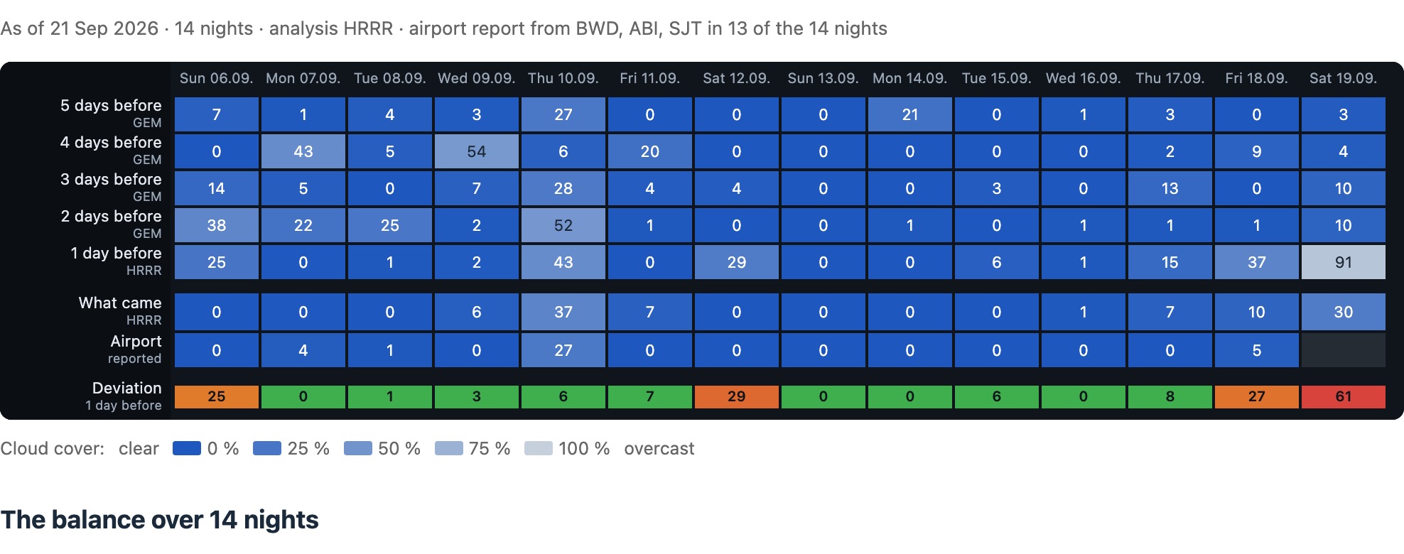
That bothered me. So I put a second page beside the astro weather, one whose whole job is to check up on it: the astro weather history. For every night of the past weeks it puts side by side what the forecast said one to five days ahead, what came of it, and what the nearby airports actually reported.
This article explains where those data come from, why the question “what actually happened?” turned out to be harder than expected – and what 60 nights at four locations say about how far the forecast can be trusted. One of the results genuinely surprised me.
How you know what was forecast
The hard part is not finding out what the weather did. The hard part is getting hold of the old forecast – what the forecast said on the Tuesday for the Friday, now that Friday is long gone. If nobody writes it down, it is gone.
Open-Meteo writes it down. The API has an endpoint for exactly this, previous-runs, and it was the discovery without which this page would not exist:
| Archive | What is in it | Reaches back |
|---|---|---|
| previous-runs | What was forecast, broken down by lead time: cloud_cover_previous_day1 to day8 | 92 days |
| The ordinary API’s own history | What came – in Texas identical to the HRRR analysis, checked hour by hour | about 70 days |
| The reanalysis archive | ERA5 at 25 km, ECMWF IFS at 9 km, CERRA at 5 km for Europe | ERA5 to 1940 |
| Airport reports | The hourly METAR cloud layers, in the archive of Iowa State University | decades |
The first three cost nothing and need no key; the fourth is a public university archive. Together they give exactly what an honest check needs: the forecast as it stood, several independent estimates of the outcome – and one real measurement.
What can not be replayed
Here I had to lower my sights. For each lead time the forecast archive carries the total cloud cover, humidity, temperature, dew point, surface wind and the weather code. It does not carry cloud cover by height, visibility, the winds at 250 and 850 hPa, or the aerosol density.
That makes two of the astro weather’s three derived rows impossible to reconstruct. Seeing is computed from the wind profile aloft – in hindsight those data do not exist broken down by lead time. Transparency comes from the CAMS aerosol forecast – the same. And without those two, the overall rating cannot be reconstructed either.
That sounds worse than it is. In the overall rating, cloud decides almost everything anyway: it enters squared, and seeing and transparency only shade an hour that is already clear. Half covered means 25 per cent at best, no matter how steady the air is. So the history compares cloud cover only – and says so on the page, rather than feigning a completeness it does not have.
The real problem: there is no single reality
I had assumed the forecast was the difficult half and that “what actually happened” was simply a fact. It is not. Cloud cover is not measured over an area; it is computed – in hindsight too. And the hindcasts disagree:
| Two hindcasts of the same period, compared | Difference |
|---|---|
| IFS analysis (9 km) against HRRR analysis (3 km) | 12.5 percentage points |
| IFS analysis against ERA5 (25 km) | 14.2 percentage points |
| ERA5 against HRRR analysis | 16.5 percentage points |
For comparison: the error of the one-day forecast at Starfront is 13 percentage points. Two of those three realities lie further apart than the forecast lies from the one I measure it against. Present one of them as “what happened” and measure everything against it, and a good part of what you are measuring is yourself.
So the page shows two references rather than one: the analysis of the finest model in the chain – and beneath it, where there is one, the airport report. That is the only real measurement in the whole arrangement: a ceilometer fires a laser pulse upwards and measures the height it is scattered back from. No model, no grid, no interpolation.
It comes with two hard limits. First, it sees only to about 3.7 km – cirrus above that, often the very thing that makes or breaks an astrophoto, does not appear in it at all. Second, it stands at the airport and not at the observatory – at the finca in Andalusia the nearest reporting airport is Gibraltar, 40 km away and at sea level while the finca sits in the mountains.
How much that matters can be measured – and it was the biggest surprise of the whole exercise. I compare the airport report with the analysis’s total cloud – over the same 60 nights from 23 July to 20 September – and look not at the size of the difference but at its direction:
| Location | Airport reads clearer than the model by |
|---|---|
| Starfront (Texas) | 0.4 percentage points |
| Finca Olivar, Gaucín | 10.0 |
| Public Observatory Hannover | 46.4 |
| Sankt Andreasberg | 48.9 |
Over dry Texas the laser and the model agree almost exactly – 0.4 percentage points across 59 nights. That is what makes the analysis a dependable reference there. In northern Germany they stand nearly fifty points apart, and that is not a measurement error: it is the mid and high cloud the ceilometer simply cannot see. In the hours where the station reports “nothing below”, the model gives on average 16 per cent low cloud but 44 per cent mid and 36 per cent high. The station is right – it just answers a different question from the one an astrophotographer asks.
Which model actually made which forecast
One point I had underestimated while building it: the forecast for “in three days” does not come from the same model as the one for tomorrow. The astro weather always takes the finest model that still reaches that far – and the fine ones do not reach far. HRRR at 3 km reaches about 48 hours out, ICON-D2 at 2.2 km much the same – enough for tomorrow night, no longer enough for the night after. After that the next coarser model takes over.
The history reproduces that very rule in hindsight: for each lead time it takes the first model in the chain that has a run at all. (This is the exact spot where the checking later changed something – more on that below.) The short-range models then drop out by themselves. This is how it came out – and it is printed on the page to the left of every row:
| Location | 1 day | 2 days | 3–4 days | 5 days |
|---|---|---|---|---|
| Starfront (Texas) | HRRR | GEM | GEM | GEM |
| Hannover, Sankt Andreasberg | ICON-D2 | ICON-EU | ICON-EU | ICON global |
| Gaucín (Andalusia) | ICON-EU | ICON-EU | ICON-EU | ICON global |
Gaucín has no high-resolution tier at all: the finca lies south of the ICON-D2 domain and south of the Danish weather service’s HARMONIE domain. For those models the API does not return zeroes there; it returns no key at all – which the chain rule handles correctly of its own accord.
And now the numbers
60 nights, 23 July to 20 September 2026. What is measured is the mean over astronomical darkness, each hour weighted by how much of it is dark – the same arithmetic the astro weather uses for its night average. A night counts only when at least 80 per cent of its darkness has data – a rule that costs a few nights at some locations, which is why the table below does not read 60 throughout.
| Location | 1 day before | 3 days before | 5 days before | usable nights |
|---|---|---|---|---|
| Starfront (Texas) | 13.0 | 6.2 | 5.9 | 59 of 60 |
| Public Observatory Hannover | 13.0 | 20.7 | 24.9 | 14 of 57 |
| Sankt Andreasberg | 11.6 | 13.8 | 25.9 | 14 of 59 |
| Finca Olivar, Gaucín | 11.2 | 14.4 | 18.9 | 39 of 59 |
Mean absolute error in percentage points of cloud cover; smaller is better. “Usable” here means under 30 per cent cover on average.
In Europe it behaves as you would expect: the further ahead, the worse – in Hannover almost a doubling of the error between one day and five. In Texas that does not happen. There the forecast gets better with a longer lead. The reason is in the last column: 59 of 60 nights were usable. In a Texas late summer, “clear” is the right answer, and you can get that right five days out too.
The one finding that surprised me
That same column makes something else visible, though, and it is the most interesting part of the whole exercise. The hit rate alone would look magnificent in Texas – 82 to 93 per cent of its calls right, depending on the lead time. Except that saying “it will be clear” every single night would score 98 per cent there. A hit rate without its base rate is worthless.
So I scored the two kinds of statement separately: promises and warnings, one at a time.
| Said three days ahead … | Starfront (Texas) | Hannover |
|---|---|---|
| “It will be usable” – and it was | 56 of 57 (98 %) | 6 of 12 (50 %) |
| “Not worth it” – and it was not | 0 of 3 (0 %) | 37 of 45 (82 %) |
That is a clean mirror image. In Texas the promises hold – and the three warnings there were turned out to be wrong, every one of them: each of those nights was usable after all. Three nights are an anecdote rather than a rate, but they point the same way as the HRRR numbers further down. In Hannover it is precisely the other way round: when it says “not worth it” there, that holds four times in five. When it says “it will be good”, it is a coin toss.
This is not a weakness in the models. It is statistics: a forecast is always good at whatever is common anyway. Predicting rare events is hard, and the rare call is the unreliable one – in Texas the bad night, in northern Germany the good one. Once you know that, you are right to read the same display differently in the two places.
And then there was HRRR
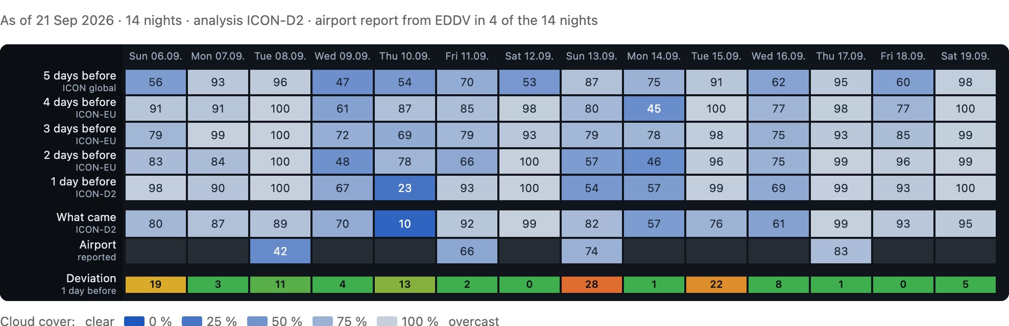
One detail in the table above I first took for an arithmetic error of mine: at Starfront the one-day forecast is worse than the three-day one. 13.0 against 6.2 percentage points – that is not a rounding difference, that is a factor of two in the wrong direction.
What differs between the two rows is the model. At one day it is HRRR doing the computing; from two days out, the Canadian GEM. And on individual nights, at the far end of its range, HRRR falls apart. The four worst cases out of the 60 nights:
| Night | 1 day before (HRRR) | 3 days before (GEM) | Actually |
|---|---|---|---|
| 20 August | 86 % | 8 % | 0 % |
| 28 August | 77 % | 0 % | 24 % |
| 4 September | 73 % | 36 % | 0 % |
| 20 September | 91 % | 10 % | 30 % |
Four times a thickly overcast night predicted – and three times it turned out clear, while the fourth (20 September) landed at exactly 30 %, right on the threshold. Had I gone by that the evening before, I would have thrown away three good nights and a usable one.
Before I believed it, I measured it again with a second, independently written tool – different night window, different reference, namely the airport reports themselves rather than the analysis. It confirms the finding: HRRR at one day’s lead 14.2 points, GEM at three days 7.3. Two routes, one answer. It is not an artefact of how I measured it.
So I rebuilt the page
That turned the question from whether to do something into what exactly. Which needed one measurement I had not actually made: HRRR against GEM at the same lead time. Until then I had only compared HRRR at one day with GEM at three – that is not a fair comparison, it is two different questions.
| Model | 0 to 24 hours | 24 to 48 hours |
|---|---|---|
| HRRR | 4.6 | 14.2 |
| GEM | 7.7 | 7.9 |
| NAM | 6.2 | 9.7 |
| NBM | 11.5 | 13.3 |
Mean error against the airport reports, 59 nights, dark hours only. Measured against the model analysis instead of the airports, the ordering comes out the same.
That settles it: HRRR is the best model there is here on the first day – and the worst of the fine ones on the second. GEM is very nearly twice as good there. So this was never about getting rid of HRRR; it was about letting go of it in time.
Since 21 September, HRRR therefore gets 30 forecast hours rather than the best part of two days, and GEM takes the rest. Why 30 and not 24: my measurement only resolves whole days, that is all the data will carry – and 30 hours stop the cut from falling in the darkest part of a night. It lands in the day that follows instead, where nothing is rated anyway.
And because I did not want to generalise from one location, I ran the same measurement for Europe. The problem is not there: at 24 to 48 hours ICON-D2 sits at 13.0 against ICON-EU’s 14.3 in Hannover, and at 11.5 against 11.2 in Sankt Andreasberg. A tie. ICON-D2 does not fall apart at the end of its range, so in Europe everything stays as it was.
Sixty nights is one late summer and not a climatology – that holds for this decision too. But at least it is a decision made from numbers rather than a hunch, and the good part is this: the history will now measure, by itself, whether it helped. In four weeks I shall know. That is exactly what I built the page for.
Where these numbers stop
- Sixty nights is not many. One late summer, one weather regime. In a Texas winter or a European blocking high the same arithmetic comes out differently.
- Cloud cover only, and of that only the total. The history says nothing about seeing and transparency – those data do not exist in hindsight.
- The reference is usually a model itself. Only at Starfront is it backed by real measurement. In Hannover and Sankt Andreasberg the airport rows are nearly empty.
- Cirrus is missing from the measurements. The ceilometer sees to 3.7 km. The thin high layer that ruins a frame without your ever noticing it in the sky appears in none of these numbers.
How the page is built
A word on the engineering. The first version queried the archives on my own machine and put the result on the server as a finished file – tidy, but with the catch that I would have had to run a script regularly. A page that is only current when its owner remembers to update it is not a good page. So it now computes live in your browser: on opening, it fetches the archived forecasts straight from Open-Meteo – one request, some 90 kilobytes, half a second – and works out the nights, the twilight and the averages on the spot. It is therefore always as current as this morning, with nobody having to do anything.
The airport reports are the special case. Iowa State University’s archive hands out one station at a time – ask for three at once and it answers “too many requests”. One after another with a pause takes six to eight seconds. That is not something to inflict on anyone merely for opening a page, nor on a free academic archive at every visit. So that row arrives only on a click.
Said plainly: this means Open-Meteo learns your IP address when the page opens, and Iowa State University learns it too if you press the button. Both are named, with their purpose and legal basis, in the privacy policy. The observing planner still does it the other way round for its orbital data – those change only every few weeks, so there the prepared file earns its keep.
Sun, moon and the exact twilight boundaries come from the same computational core the other two astronomy pages use – not from a second, slightly different copy. That sounds like housekeeping, but it is the difference between “the same night” and “roughly the same night”.
What I take away
Three things. First: a forecast without a scorecard is an assertion. It cost an afternoon to check, and I have had a distinctly different relationship with my own display ever since.
Second: you have to know what is rare where you observe. The same number means one thing at the public observatory and another in Texas – systematically so, not by chance.
Third, and the most transferable: the question “what am I actually measuring against?” was harder than the measurement. I expected to check against reality and learned instead that there are three of them, lying 12.5 to 16.5 points apart. That is no excuse for not checking. It is merely the reason why the page carries two reference rows rather than one – and why below them sits a box saying what the numbers do not mean.
To the astro weather history →
Four locations, 14 to 60 nights, free and without an account – like everything here.